Functions penguin body condition (solution)

Exercise

Body condition describes the mass of an animal relative to the mass expected given its size. Individuals that are heavier than expected are considered to be in better condition.

If the file penguins.csv is not in your working directory then download it.

Write a function called est_mass_from_flipper that takes flipper_length (in mm), a, and b as arguments. Set default arguments for a = 0.018 and b = 2.33. The function should estimate the expected body mass using mass = a * flipper_length ^ b. Use the function to estimate the expected mass of a penguin with a flipper length of 200 mm.
Write a function called calc_body_condition that takes observed_mass and expected_mass as arguments and returns the body condition, where body condition is observed_mass / expected_mass. Use the function to calculate the body condition of a penguin that weighs 4200 g but was expected to weigh 4000 g.
Load penguins.csv using read_csv(). Use mutate() and the two functions you wrote to add a new column named body_condition to the data frame.
Calculate the average body_condition for each sex of each species.
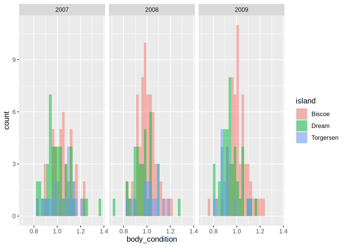
Make an unstacked histogram of body condition with the bars colored by island with one subplot (facet) for each year.

Output solution


Attaching package: 'dplyr'

The following objects are masked from 'package:stats':

    filter, lag

The following objects are masked from 'package:base':

    intersect, setdiff, setequal, union

[1] 4136.875

[1] 1.05

Rows: 344 Columns: 8
── Column specification ────────────────────────────────────────────────────────
Delimiter: ","
chr (3): species, island, sex
dbl (5): bill_length_mm, bill_depth_mm, flipper_length_mm, body_mass_g, year

ℹ Use `spec()` to retrieve the full column specification for this data.
ℹ Specify the column types or set `show_col_types = FALSE` to quiet this message.

# A tibble: 344 × 9
   species island    bill_length_mm bill_depth_mm flipper_length_mm body_mass_g
   <chr>   <chr>              <dbl>         <dbl>             <dbl>       <dbl>
 1 Adelie  Torgersen           39.1          18.7               181        3750
 2 Adelie  Torgersen           39.5          17.4               186        3800
 3 Adelie  Torgersen           40.3          18                 195        3250
 4 Adelie  Torgersen           NA            NA                  NA          NA
 5 Adelie  Torgersen           36.7          19.3               193        3450
 6 Adelie  Torgersen           39.3          20.6               190        3650
 7 Adelie  Torgersen           38.9          17.8               181        3625
 8 Adelie  Torgersen           39.2          19.6               195        4675
 9 Adelie  Torgersen           34.1          18.1               193        3475
10 Adelie  Torgersen           42            20.2               190        4250
# ℹ 334 more rows
# ℹ 3 more variables: sex <chr>, year <dbl>, body_condition <dbl>

`summarise()` has regrouped the output.
ℹ Summaries were computed grouped by species and sex.
ℹ Output is grouped by species.
ℹ Use `summarise(.groups = "drop_last")` to silence this message.
ℹ Use `summarise(.by = c(species, sex))` for per-operation grouping
  (`?dplyr::dplyr_by`) instead.

# A tibble: 6 × 3
# Groups:   species [3]
  species   sex    avg_body_condition
  <chr>     <chr>               <dbl>
1 Adelie    female              0.945
2 Adelie    male                1.07 
3 Chinstrap female              0.943
4 Chinstrap male                0.952
5 Gentoo    female              0.980
6 Gentoo    male                1.05

`stat_bin()` using `bins = 30`. Pick better value `binwidth`.

Warning: Removed 2 rows containing non-finite outside the scale range
(`stat_bin()`).