An experiment in Kenya has been exploring the influence of large herbivores on plants.
Check to see if ACACIA_DREPANOLOBIUM_SURVEY.txt is in your workspace. If not, download it. Read it into R using the following command:
acacia <-read_tsv("data/ACACIA_DREPANOLOBIUM_SURVEY.txt", na =c("dead"))
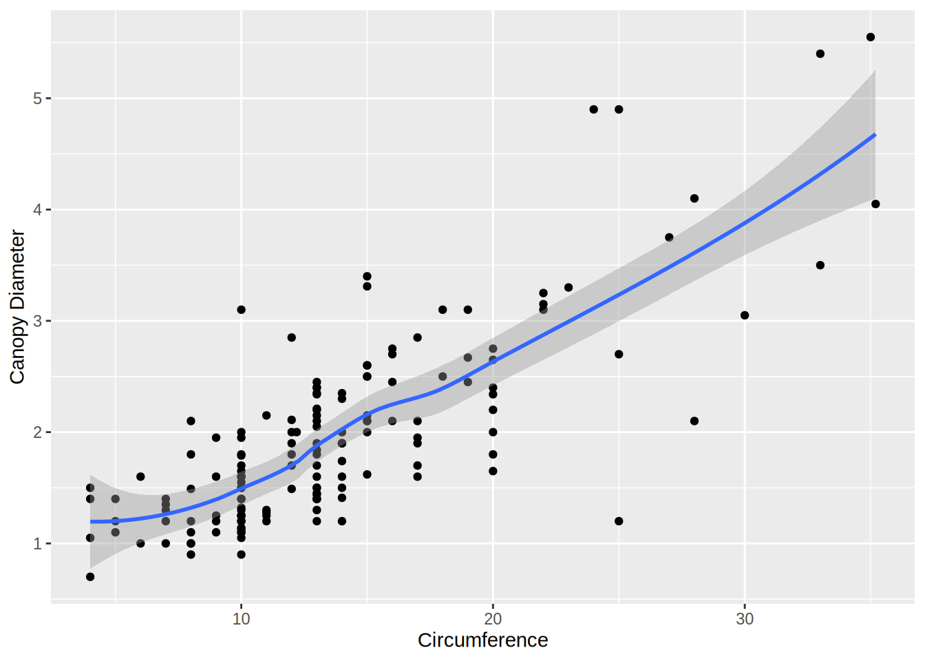
Make a scatter plot with CIRC on the x axis and AXIS1 (the maximum canopy width) on the y axis. Add a simple model of the data by adding geom_smooth. Label the x axis “Circumference” and the y axis “Canopy Diameter”.
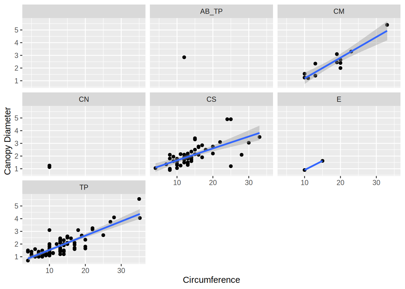
The same plot as (1), but use a linear model (method = "lm") and show different species of ant (values of ANT) in separate subplots. Once this works, you can, as an optional challenge, try to automatically include only plot subplots (i.e., ant species) with at least 5 data points. Note: results are shown for the basic exercise, not the optional challenge.
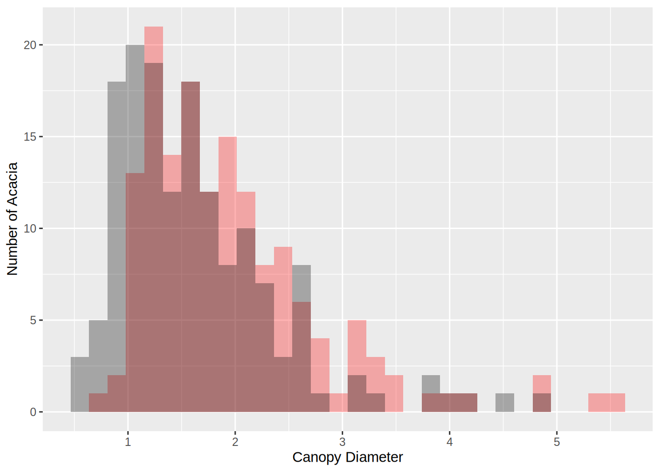
Make a plot that shows histograms of both AXIS1 and AXIS2. Due to the way the data is structured you’ll need to add a 2nd geom_histogram() layer that specifies a new aesthetic. To make it possible to see both sets of bars you’ll need to make them transparent with the optional argument alpha = 0.3. Set the color for AXIS1 to “red” and AXIS2 to “black” using the fill argument. Label the x axis “Canopy Diameter(m)” and the y axis “Number of Acacia”.
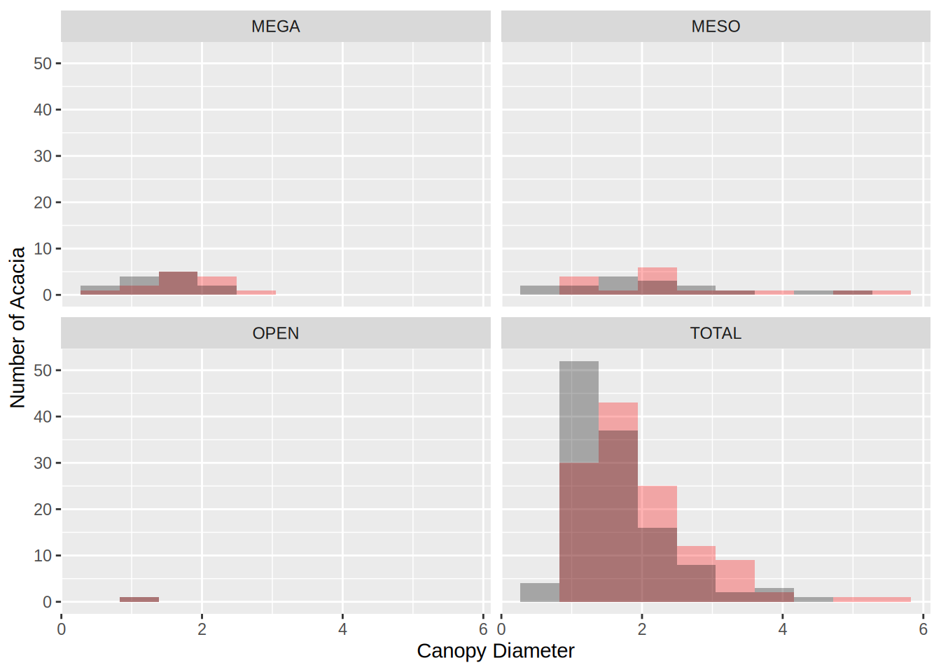
Use facet_wrap() to make the same plot as (3) but with one subplot for each treatment. Set the number of bins in the histogram to 10.
CautionOutput solution
Warning: One or more parsing issues, call `problems()` on your data frame for details,
e.g.:
  dat <- vroom(...)
  problems(dat)
Rows: 157 Columns: 15
── Column specification ────────────────────────────────────────────────────────
Delimiter: "\t"
chr  (4): SITE, TREATMENT, PLOT, ANT
dbl (11): SURVEY, YEAR, BLOCK, ID, HEIGHT, AXIS1, AXIS2, CIRC, FLOWERS, BUDS...

ℹ Use `spec()` to retrieve the full column specification for this data.
ℹ Specify the column types or set `show_col_types = FALSE` to quiet this message.
1
`geom_smooth()` using method = 'loess' and formula = 'y ~ x'
Warning: Removed 4 rows containing non-finite outside the scale range
(`stat_smooth()`).
Warning: Removed 4 rows containing missing values or values outside the scale range
(`geom_point()`).
2
`geom_smooth()` using formula = 'y ~ x'
Warning: Removed 4 rows containing non-finite outside the scale range
(`stat_smooth()`).
Warning in qt((1 - level)/2, df): NaNs produced
Warning: Removed 4 rows containing missing values or values outside the scale range
(`geom_point()`).
Warning in max(ids, na.rm = TRUE): no non-missing arguments to max; returning
-Inf
3
`stat_bin()` using `bins = 30`. Pick better value `binwidth`.
Warning: Removed 4 rows containing non-finite outside the scale range
(`stat_bin()`).
`stat_bin()` using `bins = 30`. Pick better value `binwidth`.
Warning: Removed 4 rows containing non-finite outside the scale range
(`stat_bin()`).
4
Warning: Removed 4 rows containing non-finite outside the scale range (`stat_bin()`).
Removed 4 rows containing non-finite outside the scale range (`stat_bin()`).