Graphing acacia ants data manip.qmd (solution)

Exercise

An experiment in Kenya has been exploring the influence of large herbivores on plants.

Check to see if ACACIA_DREPANOLOBIUM_SURVEY.txt and TREE_SURVEYS.txt is in your workspace. If not, download ACACIA_DREPANOLOBIUM_SURVEY.txt and TREE_SURVEYS.txt Install the readr package and use read_tsv to read in the data using the following commands:

library(readr)
acacia <- read_tsv("ACACIA_DREPANOLOBIUM_SURVEY.txt", na = c("dead"))
trees <- read_tsv("TREE_SURVEYS.txt",
                  col_types = list(HEIGHT = col_double(),
                                   AXIS_2 = col_double()))

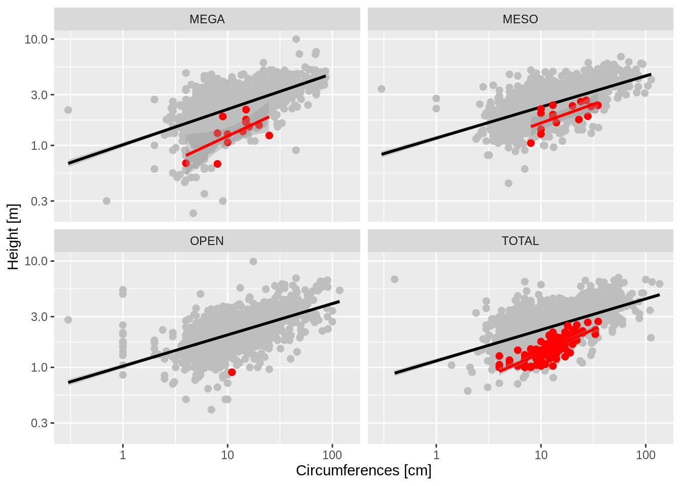
We want to compare the circumference to height relationship in acacia on different treatments in the context of the same relationship for trees in the region. These data are stored in the two tables above. Make a graph with the relationship between CIRC and HEIGHT for the trees as gray points in the background and the same relationship for acacia as red points plotted on top of the tree points. There should be one subplot for each treatment. Scale the both axes logarithmically. Include linear models for both sets of data. Provide clear labels for the axes.

Output solution

Code solution for Graphing Acacia and Ants Data Manipulation

Attaching package: 'dplyr'

The following objects are masked from 'package:stats':

    filter, lag

The following objects are masked from 'package:base':

    intersect, setdiff, setequal, union

Warning: One or more parsing issues, call `problems()` on your data frame for details,
e.g.:
  dat <- vroom(...)
  problems(dat)

Rows: 157 Columns: 15

── Column specification ────────────────────────────────────────────────────────
Delimiter: "\t"
chr  (4): SITE, TREATMENT, PLOT, ANT
dbl (11): SURVEY, YEAR, BLOCK, ID, HEIGHT, AXIS1, AXIS2, CIRC, FLOWERS, BUDS...

ℹ Use `spec()` to retrieve the full column specification for this data.
ℹ Specify the column types or set `show_col_types = FALSE` to quiet this message.

Warning: One or more parsing issues, call `problems()` on your data frame for details,
e.g.:
  dat <- vroom(...)
  problems(dat)

`geom_smooth()` using formula = 'y ~ x'

Warning: Removed 407 rows containing non-finite outside the scale range
(`stat_smooth()`).

`geom_smooth()` using formula = 'y ~ x'

Warning: Removed 4 rows containing non-finite outside the scale range
(`stat_smooth()`).

Warning: Removed 407 rows containing missing values or values outside the scale range
(`geom_point()`).

Warning: Removed 4 rows containing missing values or values outside the scale range
(`geom_point()`).